ch2 - 머신러닝 프로젝트 처음부터 끝까지
이제부터 나는 부동산 회사에 막 고용된 데이터 사이언티스트이다.
내가 할 일은 '캘리포니아 인구조사 데이터'를 사용해 캘리포니아의 구역 별 중간 주택 가격 예측 모델을 만들어야 한다.
데이터가 담고있는 정보:
- 블록 그룹(block group, 혹은 구역)마다 인구(population)
- 중간 소득(median income)
- 중간 주택 가격(median housing price)
- etc...
크게 아래와 같이 진행 예정
- 큰 그림 보기
- 데이터 구하기
- 데이터로부터 패턴을 파악하기 위해 탐색 및 시각화
- 머신러닝 알고리즘을 위한 데이터 준비
- 모델 선택 및 훈련
- 모델 상세히 조정
- 솔루션(문제 해결 방법) 제시
- 시스템 런칭 및 모니터링, 유지 보수
문제 정의
문제를 정의하기 전, 설계를 위한 정보가 필요함
'비즈니스의 목적이 정확히 무엇인가?'
- 해당 모델을 어떻게 사용해 이익을 얻으려고 하는가
- 문제 구성, 어떤 알고리즘 선택, 모델 평가에 어떤 성능 지표 사용할 지, 모델 튜닝 위해 얼마나 노력 투여할 지 결정 위해 중요한 질문
'현재 문제 해결 방법은 어떻게 구성되어 있는가?'
- 머신러닝 모델이 사용되고 있지 않은 지금은 어떻게 문제를 해결하고 있는가 (참고용)
- ex) 현재 구역 별 중간 주택 가격 예측은 전문가가 수동으로 하고 있으며, 전문가의 추정 가격은 실제 주택 가격의 10% 정도가 벗어나는 문제가 있음.
- 이는 구역의 데이터를 기반으로 중간 주택 가격을 예측하는 모델을 훈련시키는 쪽이 유용할 듯 함.
정보를 얻었으니 문제를 정의하여 설계를 해보자.
우리가 만들 시스템은 어떤 학습 방법을 사용하게 될까?
- 지도 학습? 비지도 학습? 강화 학습?
- 분류 및 회귀? 기타 다른 방법?
- 배치 학습? 온라인 학습?
우리 예제에서는 '레이블'된 훈련 샘플이 존재(각 value 별 정답으로 '기대 출력값(구역의 중간 주택 가격)'을 가지고 있음)
-> 따라서 '지도 학습'이 적합할 듯
또한 정해진 정답(레이블) 내에서 새로운 값의 소속을 분류 하는 것이 아님. 새로운 값이 새로운 정답(타깃 수치)으로 예측 되어야 해.
-> 따라서 '회귀'가 적합할 듯, 그런데 feature가 많으므로 '다변량 회귀'가 가장 적합할 듯
시스템으로 들어오는 데이터에 연속적인 흐름이 없고 빠르게 변하는 데이터에 적응할 필요가 일단은 없음. 메모리도 작아
-> '배치 학습'이 적절
성능 측정 지표 선택
흔히 Loss function이라 불리는 것으로 어떤 것을 선택하는지에 대한 문제이며, 여러 함수가 있으나 자세한 수학적인 설명은 일단 제외.
Loss function(손실 함수)이란 훈련하면서 도출된 예측 값을 실제 값(레이블)과 비교할 때 사용하는 함수이며, 해당 함수 적용의 결과 값이 작을 수록 오차가 적은 것임.
회귀 문제에서는 보통 '평균 제곱근 오차(Root Mean Square Error, RMSE)'를 사용하므로 해당 함수를 사용할 것임.
$RMSE(X,h)=\sqrt{\frac{1}{m}\sum_{i=1}^{m}{(h(x^{(i)})-y^{(i)}})^2}$
이제 데이터를 구하여 가져와 보자
# 파이썬 2와 파이썬 3 지원
from __future__ import division, print_function, unicode_literals

# 공통
import numpy as np
import os

# 일관된 출력을 위해 유사난수 초기화
np.random.seed(42)

# 맷플롯립 설정
%matplotlib inline
import matplotlib
import matplotlib.pyplot as plt
plt.rcParams['axes.labelsize'] = 14
plt.rcParams['xtick.labelsize'] = 12
plt.rcParams['ytick.labelsize'] = 12

# 한글출력
matplotlib.rc('font', family='NanumBarunGothic')
plt.rcParams['axes.unicode_minus'] = False

# 그림을 저장할 폴드
PROJECT_ROOT_DIR = "."
CHAPTER_ID = "end_to_end_project"
IMAGES_PATH = os.path.join(PROJECT_ROOT_DIR, "images", CHAPTER_ID)

def save_fig(fig_id, tight_layout=True, fig_extension="png", resolution=300):
    path = os.path.join(IMAGES_PATH, fig_id + "." + fig_extension)
    if tight_layout:
        plt.tight_layout()
    plt.savefig(path, format=fig_extension, dpi=resolution)
import os
import tarfile
from six.moves import urllib

DOWNLOAD_ROOT = "https://raw.githubusercontent.com/ageron/handson-ml/master/"
HOUSING_PATH = os.path.join("datasets", "housing")
HOUSING_URL = DOWNLOAD_ROOT + "datasets/housing/housing.tgz"

def fetch_housing_data(housing_url=HOUSING_URL, housing_path=HOUSING_PATH):
    if not os.path.isdir(housing_path):
        os.makedirs(housing_path)
    tgz_path = os.path.join(housing_path, "housing.tgz")
    urllib.request.urlretrieve(housing_url, tgz_path)
    housing_tgz = tarfile.open(tgz_path)
    housing_tgz.extractall(path=housing_path)
    housing_tgz.close()
fetch_housing_data()
import pandas as pd

def load_housing_data(housing_path=HOUSING_PATH):
    csv_path = os.path.join(housing_path, "housing.csv")
    return pd.read_csv(csv_path)
데이터를 불러왔으니 데이터를 훑어보자
housing = load_housing_data()
housing.head()
| longitude | latitude | housing_median_age | total_rooms | total_bedrooms | population | households | median_income | median_house_value | ocean_proximity | |
|---|---|---|---|---|---|---|---|---|---|---|
| 0 | -122.23 | 37.88 | 41.0 | 880.0 | 129.0 | 322.0 | 126.0 | 8.3252 | 452600.0 | NEAR BAY |
| 1 | -122.22 | 37.86 | 21.0 | 7099.0 | 1106.0 | 2401.0 | 1138.0 | 8.3014 | 358500.0 | NEAR BAY |
| 2 | -122.24 | 37.85 | 52.0 | 1467.0 | 190.0 | 496.0 | 177.0 | 7.2574 | 352100.0 | NEAR BAY |
| 3 | -122.25 | 37.85 | 52.0 | 1274.0 | 235.0 | 558.0 | 219.0 | 5.6431 | 341300.0 | NEAR BAY |
| 4 | -122.25 | 37.85 | 52.0 | 1627.0 | 280.0 | 565.0 | 259.0 | 3.8462 | 342200.0 | NEAR BAY |
housing.info()
<class 'pandas.core.frame.DataFrame'>
RangeIndex: 20640 entries, 0 to 20639
Data columns (total 10 columns):
 #   Column              Non-Null Count  Dtype
---  ------              --------------  -----
 0   longitude           20640 non-null  float64
 1   latitude            20640 non-null  float64
 2   housing_median_age  20640 non-null  float64
 3   total_rooms         20640 non-null  float64
 4   total_bedrooms      20433 non-null  float64
 5   population          20640 non-null  float64
 6   households          20640 non-null  float64
 7   median_income       20640 non-null  float64
 8   median_house_value  20640 non-null  float64
 9   ocean_proximity     20640 non-null  object
dtypes: float64(9), object(1)
memory usage: 1.6+ MB
housing["ocean_proximity"].value_counts()
<1H OCEAN     9136
INLAND        6551
NEAR OCEAN    2658
NEAR BAY      2290
ISLAND           5
Name: ocean_proximity, dtype: int64
housing.describe()
| longitude | latitude | housing_median_age | total_rooms | total_bedrooms | population | households | median_income | median_house_value | |
|---|---|---|---|---|---|---|---|---|---|
| count | 20640.000000 | 20640.000000 | 20640.000000 | 20640.000000 | 20433.000000 | 20640.000000 | 20640.000000 | 20640.000000 | 20640.000000 |
| mean | -119.569704 | 35.631861 | 28.639486 | 2635.763081 | 537.870553 | 1425.476744 | 499.539680 | 3.870671 | 206855.816909 |
| std | 2.003532 | 2.135952 | 12.585558 | 2181.615252 | 421.385070 | 1132.462122 | 382.329753 | 1.899822 | 115395.615874 |
| min | -124.350000 | 32.540000 | 1.000000 | 2.000000 | 1.000000 | 3.000000 | 1.000000 | 0.499900 | 14999.000000 |
| 25% | -121.800000 | 33.930000 | 18.000000 | 1447.750000 | 296.000000 | 787.000000 | 280.000000 | 2.563400 | 119600.000000 |
| 50% | -118.490000 | 34.260000 | 29.000000 | 2127.000000 | 435.000000 | 1166.000000 | 409.000000 | 3.534800 | 179700.000000 |
| 75% | -118.010000 | 37.710000 | 37.000000 | 3148.000000 | 647.000000 | 1725.000000 | 605.000000 | 4.743250 | 264725.000000 |
| max | -114.310000 | 41.950000 | 52.000000 | 39320.000000 | 6445.000000 | 35682.000000 | 6082.000000 | 15.000100 | 500001.000000 |
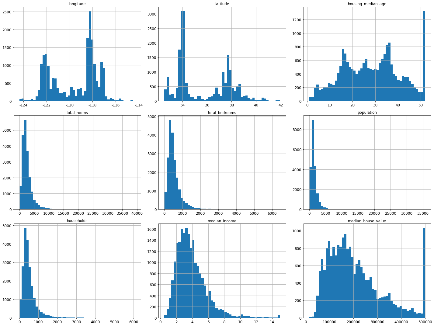
%matplotlib inline
import matplotlib.pyplot as plt
housing.hist(bins=50, figsize=(20,15))
save_fig("attribute_histogram_plots")
plt.show()
findfont: Font family ['NanumBarunGothic'] not found. Falling back to DejaVu Sans.


---------------------------------------------------------------------------
# 일관된 출력을 위해 유사난수 초기화
np.random.seed(42)
테스트 데이터 셋 만들기
이전에 알아봤듯이 우리는 데이터셋이 크게 '훈련 데이터'와 '시험(테스트) 데이터'로 나뉜다는 것을 안다.
전체 데이터셋에서 훈련 데이터로 사용하는 친구들은 정답(중간 소득)과 함께 하고, 시험 데이터로 사용하는 친구들은 정답을 제거하고 사용하게 된다.
제거한 정답은 버리는게 아니라, 시험 데이터를 통해 예측된 값과 비교하여 오차를 계산하는데에 사용된다.
import numpy as np

# 예시를 위해서 만든 것입니다. 사이킷런에는 train_test_split() 함수가 있습니다.
def split_train_test(data, test_ratio):
    shuffled_indices = np.random.permutation(len(data))
    test_set_size = int(len(data) * test_ratio)
    test_indices = shuffled_indices[:test_set_size]
    train_indices = shuffled_indices[test_set_size:]
    return data.iloc[train_indices], data.iloc[test_indices]
train_set, test_set = split_train_test(housing, 0.2)
print(len(train_set), "train +", len(test_set), "test")
16512 train + 4128 test
from zlib import crc32

def test_set_check(identifier, test_ratio):
    return crc32(np.int64(identifier)) & 0xffffffff < test_ratio * 2**32

def split_train_test_by_id(data, test_ratio, id_column):
    ids = data[id_column]
    in_test_set = ids.apply(lambda id_: test_set_check(id_, test_ratio))
    return data.loc[~in_test_set], data.loc[in_test_set]
import hashlib

def test_set_check(identifier, test_ratio, hash=hashlib.md5):
    return bytearray(hash(np.int64(identifier)).digest())[-1] < 256 * test_ratio
# 이 버전의 test_set_check() 함수가 파이썬 2도 지원합니다.
def test_set_check(identifier, test_ratio, hash=hashlib.md5):
    return bytearray(hash(np.int64(identifier)).digest())[-1] < 256 * test_ratio
housing_with_id = housing.reset_index()   # `index` 열이 추가된 데이터프레임이 반환됩니다.
train_set, test_set = split_train_test_by_id(housing_with_id, 0.2, "index")
housing_with_id["id"] = housing["longitude"] * 1000 + housing["latitude"]
train_set, test_set = split_train_test_by_id(housing_with_id, 0.2, "id")
test_set.head()
| index | longitude | latitude | housing_median_age | total_rooms | total_bedrooms | population | households | median_income | median_house_value | ocean_proximity | id | |
|---|---|---|---|---|---|---|---|---|---|---|---|---|
| 8 | 8 | -122.26 | 37.84 | 42.0 | 2555.0 | 665.0 | 1206.0 | 595.0 | 2.0804 | 226700.0 | NEAR BAY | -122222.16 |
| 10 | 10 | -122.26 | 37.85 | 52.0 | 2202.0 | 434.0 | 910.0 | 402.0 | 3.2031 | 281500.0 | NEAR BAY | -122222.15 |
| 11 | 11 | -122.26 | 37.85 | 52.0 | 3503.0 | 752.0 | 1504.0 | 734.0 | 3.2705 | 241800.0 | NEAR BAY | -122222.15 |
| 12 | 12 | -122.26 | 37.85 | 52.0 | 2491.0 | 474.0 | 1098.0 | 468.0 | 3.0750 | 213500.0 | NEAR BAY | -122222.15 |
| 13 | 13 | -122.26 | 37.84 | 52.0 | 696.0 | 191.0 | 345.0 | 174.0 | 2.6736 | 191300.0 | NEAR BAY | -122222.16 |
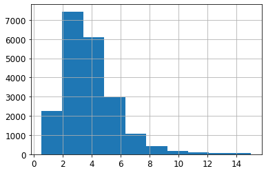
housing["median_income"].hist()
<AxesSubplot:>
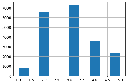
# 소득 카테고리 개수를 제한하기 위해 1.5로 나눕니다.
housing["income_cat"] = np.ceil(housing["median_income"] / 1.5)
# 5 이상은 5로 레이블합니다.
housing["income_cat"].where(housing["income_cat"] < 5, 5.0, inplace=True)
housing["income_cat"].value_counts()
3.0    7236
2.0    6581
4.0    3639
5.0    2362
1.0     822
Name: income_cat, dtype: int64
housing["income_cat"].hist()
save_fig('income_category_hist')
---------------------------------------------------------------------------
사이킷런 모듈은 데이터셋을 훈련용, 시험용으로 나누는 다양한 방법을 제공한다고 함
from sklearn.model_selection import StratifiedShuffleSplit

split = StratifiedShuffleSplit(n_splits=1, test_size=0.2, random_state=42)
for train_index, test_index in split.split(housing, housing["income_cat"]):
    strat_train_set = housing.loc[train_index]
    strat_test_set = housing.loc[test_index]
strat_test_set["income_cat"].value_counts() / len(strat_test_set)
3.0    0.350533
2.0    0.318798
4.0    0.176357
5.0    0.114341
1.0    0.039971
Name: income_cat, dtype: float64
housing["income_cat"].value_counts() / len(housing)
3.0    0.350581
2.0    0.318847
4.0    0.176308
5.0    0.114438
1.0    0.039826
Name: income_cat, dtype: float64
from sklearn.model_selection import train_test_split
def income_cat_proportions(data):
    return data["income_cat"].value_counts() / len(data)

train_set, test_set = train_test_split(housing, test_size=0.2, random_state=42)

compare_props = pd.DataFrame({
    "Overall": income_cat_proportions(housing),
    "Stratified": income_cat_proportions(strat_test_set),
    "Random": income_cat_proportions(test_set),
}).sort_index()
compare_props["Rand. %error"] = 100 * compare_props["Random"] / compare_props["Overall"] - 100
compare_props["Strat. %error"] = 100 * compare_props["Stratified"] / compare_props["Overall"] - 100
compare_props
| Overall | Stratified | Random | Rand. %error | Strat. %error | |
|---|---|---|---|---|---|
| 1.0 | 0.039826 | 0.039971 | 0.040213 | 0.973236 | 0.364964 |
| 2.0 | 0.318847 | 0.318798 | 0.324370 | 1.732260 | -0.015195 |
| 3.0 | 0.350581 | 0.350533 | 0.358527 | 2.266446 | -0.013820 |
| 4.0 | 0.176308 | 0.176357 | 0.167393 | -5.056334 | 0.027480 |
| 5.0 | 0.114438 | 0.114341 | 0.109496 | -4.318374 | -0.084674 |
for set_ in (strat_train_set, strat_test_set):
    set_.drop("income_cat", axis=1, inplace=True)
데이터 이해를 위한 탐색과 시각화
데이터를 시각적으로 보고 패턴을 대략적으로 분석해보자
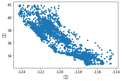
housing = strat_train_set.copy()
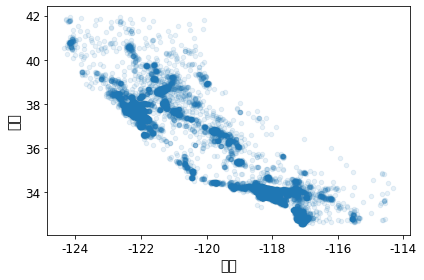
ax = housing.plot(kind="scatter", x="longitude", y="latitude")
ax.set(xlabel='경도', ylabel='위도')
save_fig("bad_visualization_plot")
# 밀집된 지역을 보다 잘 보여주는 산점도
ax = housing.plot(kind="scatter", x="longitude", y="latitude", alpha=0.1)
ax.set(xlabel='경도', ylabel='위도')
save_fig("better_visualization_plot")
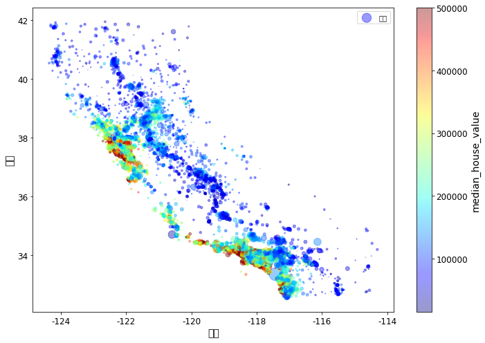
# 낮은 가격: 파란색 -> 높은 가격: 빨간색
ax = housing.plot(kind="scatter", x="longitude", y="latitude", alpha=0.4,
    s=housing["population"]/100, label="인구", figsize=(10,7),
    c="median_house_value", cmap=plt.get_cmap("jet"), colorbar=True,
    sharex=False)
ax.set(xlabel='경도', ylabel='위도')
plt.legend()
save_fig("housing_prices_scatterplot")
상관관계 조사
corr_matrix = housing.corr()
corr_matrix["median_house_value"].sort_values(ascending=False)
median_house_value    1.000000
median_income         0.687151
total_rooms           0.135140
housing_median_age    0.114146
households            0.064590
total_bedrooms        0.047781
population           -0.026882
longitude            -0.047466
latitude             -0.142673
Name: median_house_value, dtype: float64
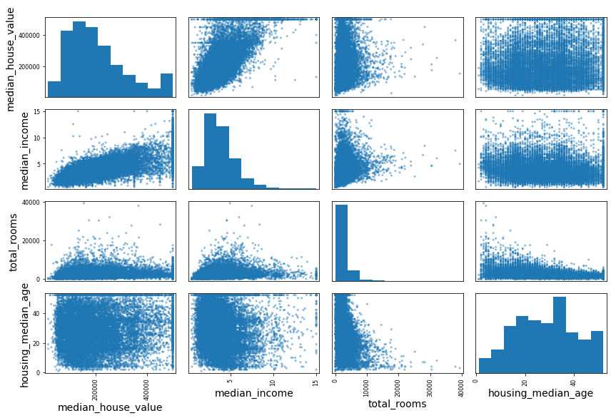
from pandas.plotting import scatter_matrix

attributes = ["median_house_value", "median_income", "total_rooms",
              "housing_median_age"]
scatter_matrix(housing[attributes], figsize=(12, 8))
save_fig("scatter_matrix_plot")
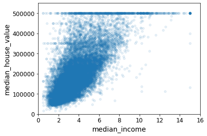
housing.plot(kind="scatter", x="median_income", y="median_house_value",
             alpha=0.1)
plt.axis([0, 16, 0, 550000])
save_fig("income_vs_house_value_scatterplot")
---------------------------------------------------------------------------
housing["rooms_per_household"] = housing["total_rooms"]/housing["households"]
housing["bedrooms_per_room"] = housing["total_bedrooms"]/housing["total_rooms"]
housing["population_per_household"]=housing["population"]/housing["households"]
corr_matrix = housing.corr()
corr_matrix["median_house_value"].sort_values(ascending=False)
median_house_value          1.000000
median_income               0.687151
rooms_per_household         0.146255
total_rooms                 0.135140
housing_median_age          0.114146
households                  0.064590
total_bedrooms              0.047781
population_per_household   -0.021991
population                 -0.026882
longitude                  -0.047466
latitude                   -0.142673
bedrooms_per_room          -0.259952
Name: median_house_value, dtype: float64
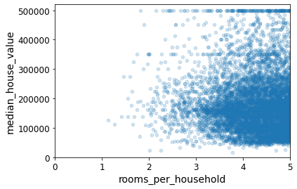
housing.plot(kind="scatter", x="rooms_per_household", y="median_house_value",
             alpha=0.2)
plt.axis([0, 5, 0, 520000])
plt.show()
housing.describe()
| longitude | latitude | housing_median_age | total_rooms | total_bedrooms | population | households | median_income | median_house_value | rooms_per_household | bedrooms_per_room | population_per_household | |
|---|---|---|---|---|---|---|---|---|---|---|---|---|
| count | 16512.000000 | 16512.000000 | 16512.000000 | 16512.000000 | 16354.000000 | 16512.000000 | 16512.000000 | 16512.000000 | 16512.000000 | 16512.000000 | 16354.000000 | 16512.000000 |
| mean | -119.575635 | 35.639314 | 28.653404 | 2622.539789 | 534.914639 | 1419.687379 | 497.011810 | 3.875884 | 207005.322372 | 5.440406 | 0.212873 | 3.096469 |
| std | 2.001828 | 2.137963 | 12.574819 | 2138.417080 | 412.665649 | 1115.663036 | 375.696156 | 1.904931 | 115701.297250 | 2.611696 | 0.057378 | 11.584825 |
| min | -124.350000 | 32.540000 | 1.000000 | 6.000000 | 2.000000 | 3.000000 | 2.000000 | 0.499900 | 14999.000000 | 1.130435 | 0.100000 | 0.692308 |
| 25% | -121.800000 | 33.940000 | 18.000000 | 1443.000000 | 295.000000 | 784.000000 | 279.000000 | 2.566950 | 119800.000000 | 4.442168 | 0.175304 | 2.431352 |
| 50% | -118.510000 | 34.260000 | 29.000000 | 2119.000000 | 433.000000 | 1164.000000 | 408.000000 | 3.541550 | 179500.000000 | 5.232342 | 0.203027 | 2.817661 |
| 75% | -118.010000 | 37.720000 | 37.000000 | 3141.000000 | 644.000000 | 1719.000000 | 602.000000 | 4.745325 | 263900.000000 | 6.056361 | 0.239816 | 3.281420 |
| max | -114.310000 | 41.950000 | 52.000000 | 39320.000000 | 6210.000000 | 35682.000000 | 5358.000000 | 15.000100 | 500001.000000 | 141.909091 | 1.000000 | 1243.333333 |
머신러닝 알고리즘을 위한 데이터 준비
흔히 데이터 전처리(pre-processing)이라고 하는 과정.
이전에 쓰레기 값을 넣으면 쓰레기 결과가 나온다는 비유를 한 적이 있으며, 쓰레기 값을 쓸모 있는 값으로 바꾸기 위한 과정임.
데이터 정제
전체 데이터에서 일부 데이터의 경우 어떤 특성(feature)에 대한 값이 누락되는 경우가 있다. 이 때 아래와 같은 행동을 취할 수 있는데, 이는 상황 by 상황으로 취하면 된다.
- 해당 데이터(row)를 아예 삭제하기
- 누락된 값이 있는 특성(feature, column)을 아예 삭제하기
- 어떤 값으로 채우기(0, 평균, 중간값 등)
housing = strat_train_set.drop("median_house_value", axis=1) # 훈련 세트를 위해 레이블 삭제
housing_labels = strat_train_set["median_house_value"].copy()
sample_incomplete_rows = housing[housing.isnull().any(axis=1)].head()
sample_incomplete_rows
| longitude | latitude | housing_median_age | total_rooms | total_bedrooms | population | households | median_income | ocean_proximity | |
|---|---|---|---|---|---|---|---|---|---|
| 1606 | -122.08 | 37.88 | 26.0 | 2947.0 | NaN | 825.0 | 626.0 | 2.9330 | NEAR BAY |
| 10915 | -117.87 | 33.73 | 45.0 | 2264.0 | NaN | 1970.0 | 499.0 | 3.4193 | <1H OCEAN |
| 19150 | -122.70 | 38.35 | 14.0 | 2313.0 | NaN | 954.0 | 397.0 | 3.7813 | <1H OCEAN |
| 4186 | -118.23 | 34.13 | 48.0 | 1308.0 | NaN | 835.0 | 294.0 | 4.2891 | <1H OCEAN |
| 16885 | -122.40 | 37.58 | 26.0 | 3281.0 | NaN | 1145.0 | 480.0 | 6.3580 | NEAR OCEAN |
sample_incomplete_rows.dropna(subset=["total_bedrooms"]) # 옵션 1
| longitude | latitude | housing_median_age | total_rooms | total_bedrooms | population | households | median_income | ocean_proximity |
|---|
sample_incomplete_rows.drop("total_bedrooms", axis=1) # 옵션 2
| longitude | latitude | housing_median_age | total_rooms | population | households | median_income | ocean_proximity | |
|---|---|---|---|---|---|---|---|---|
| 1606 | -122.08 | 37.88 | 26.0 | 2947.0 | 825.0 | 626.0 | 2.9330 | NEAR BAY |
| 10915 | -117.87 | 33.73 | 45.0 | 2264.0 | 1970.0 | 499.0 | 3.4193 | <1H OCEAN |
| 19150 | -122.70 | 38.35 | 14.0 | 2313.0 | 954.0 | 397.0 | 3.7813 | <1H OCEAN |
| 4186 | -118.23 | 34.13 | 48.0 | 1308.0 | 835.0 | 294.0 | 4.2891 | <1H OCEAN |
| 16885 | -122.40 | 37.58 | 26.0 | 3281.0 | 1145.0 | 480.0 | 6.3580 | NEAR OCEAN |
median = housing["total_bedrooms"].median()
sample_incomplete_rows["total_bedrooms"].fillna(median, inplace=True) # 옵션 3
sample_incomplete_rows
| longitude | latitude | housing_median_age | total_rooms | total_bedrooms | population | households | median_income | ocean_proximity | |
|---|---|---|---|---|---|---|---|---|---|
| 1606 | -122.08 | 37.88 | 26.0 | 2947.0 | 433.0 | 825.0 | 626.0 | 2.9330 | NEAR BAY |
| 10915 | -117.87 | 33.73 | 45.0 | 2264.0 | 433.0 | 1970.0 | 499.0 | 3.4193 | <1H OCEAN |
| 19150 | -122.70 | 38.35 | 14.0 | 2313.0 | 433.0 | 954.0 | 397.0 | 3.7813 | <1H OCEAN |
| 4186 | -118.23 | 34.13 | 48.0 | 1308.0 | 433.0 | 835.0 | 294.0 | 4.2891 | <1H OCEAN |
| 16885 | -122.40 | 37.58 | 26.0 | 3281.0 | 433.0 | 1145.0 | 480.0 | 6.3580 | NEAR OCEAN |
#from sklearn.preprocessing import Imputer
from sklearn.impute import SimpleImputer

imputer = SimpleImputer(strategy="median")
housing_num = housing.drop('ocean_proximity', axis=1)
# 다른 방법: housing_num = housing.select_dtypes(include=[np.number])
imputer.fit(housing_num)
SimpleImputer(strategy='median')
imputer.statistics_
array([-118.51   ,   34.26   ,   29.     , 2119.     ,  433.     ,
       1164.     ,  408.     ,    3.54155])
housing_num.median().values
array([-118.51   ,   34.26   ,   29.     , 2119.     ,  433.     ,
       1164.     ,  408.     ,    3.54155])
X = imputer.transform(housing_num)
housing_tr = pd.DataFrame(X, columns=housing_num.columns,
                          index = list(housing.index.values))
housing_tr.loc[sample_incomplete_rows.index.values]
| longitude | latitude | housing_median_age | total_rooms | total_bedrooms | population | households | median_income | |
|---|---|---|---|---|---|---|---|---|
| 1606 | -122.08 | 37.88 | 26.0 | 2947.0 | 433.0 | 825.0 | 626.0 | 2.9330 |
| 10915 | -117.87 | 33.73 | 45.0 | 2264.0 | 433.0 | 1970.0 | 499.0 | 3.4193 |
| 19150 | -122.70 | 38.35 | 14.0 | 2313.0 | 433.0 | 954.0 | 397.0 | 3.7813 |
| 4186 | -118.23 | 34.13 | 48.0 | 1308.0 | 433.0 | 835.0 | 294.0 | 4.2891 |
| 16885 | -122.40 | 37.58 | 26.0 | 3281.0 | 433.0 | 1145.0 | 480.0 | 6.3580 |
imputer.strategy
'median'
housing_tr = pd.DataFrame(X, columns=housing_num.columns)
housing_tr.head()
| longitude | latitude | housing_median_age | total_rooms | total_bedrooms | population | households | median_income | |
|---|---|---|---|---|---|---|---|---|
| 0 | -121.46 | 38.52 | 29.0 | 3873.0 | 797.0 | 2237.0 | 706.0 | 2.1736 |
| 1 | -117.23 | 33.09 | 7.0 | 5320.0 | 855.0 | 2015.0 | 768.0 | 6.3373 |
| 2 | -119.04 | 35.37 | 44.0 | 1618.0 | 310.0 | 667.0 | 300.0 | 2.8750 |
| 3 | -117.13 | 32.75 | 24.0 | 1877.0 | 519.0 | 898.0 | 483.0 | 2.2264 |
| 4 | -118.70 | 34.28 | 27.0 | 3536.0 | 646.0 | 1837.0 | 580.0 | 4.4964 |
텍스트와 범주형 특성 다루기
앞선 범주형 특성 ocean_proximity는 텍스트라 중간값을 계산할 수가 없었다.
텍스트가 값인 경우, 해당 값을 텍스트에서 숫자로 바꿔주는 것이 일반적이다. (mapping)
housing_cat = housing['ocean_proximity']
housing_cat.head(10)
12655        INLAND
15502    NEAR OCEAN
2908         INLAND
14053    NEAR OCEAN
20496     <1H OCEAN
1481       NEAR BAY
18125     <1H OCEAN
5830      <1H OCEAN
17989     <1H OCEAN
4861      <1H OCEAN
Name: ocean_proximity, dtype: object
housing_cat_encoded, housing_categories = housing_cat.factorize()
housing_cat_encoded[:10]
array([0, 1, 0, 1, 2, 3, 2, 2, 2, 2])
housing_categories
Index(['INLAND', 'NEAR OCEAN', '<1H OCEAN', 'NEAR BAY', 'ISLAND'], dtype='object')
from sklearn.preprocessing import OneHotEncoder

encoder = OneHotEncoder(categories='auto')
housing_cat_1hot = encoder.fit_transform(housing_cat_encoded.reshape(-1,1))
housing_cat_1hot
<16512x5 sparse matrix of type '<class 'numpy.float64'>'
    with 16512 stored elements in Compressed Sparse Row format>
housing_cat_1hot.toarray()
array([[1., 0., 0., 0., 0.],
       [0., 1., 0., 0., 0.],
       [1., 0., 0., 0., 0.],
       ...,
       [0., 0., 1., 0., 0.],
       [0., 0., 1., 0., 0.],
       [1., 0., 0., 0., 0.]])
# [PR #9151](https://github.com/scikit-learn/scikit-learn/pull/9151)에서 가져온 CategoricalEncoder 클래스의 정의.
# 이 클래스는 사이킷런 0.20에 포함될 예정입니다.

from sklearn.base import BaseEstimator, TransformerMixin
from sklearn.utils import check_array
from sklearn.preprocessing import LabelEncoder
from scipy import sparse

class CategoricalEncoder(BaseEstimator, TransformerMixin):
    """Encode categorical features as a numeric array.
    The input to this transformer should be a matrix of integers or strings,
    denoting the values taken on by categorical (discrete) features.
    The features can be encoded using a one-hot aka one-of-K scheme
    (``encoding='onehot'``, the default) or converted to ordinal integers
    (``encoding='ordinal'``).
    This encoding is needed for feeding categorical data to many scikit-learn
    estimators, notably linear models and SVMs with the standard kernels.
    Read more in the :ref:`User Guide `.
    Parameters
    ----------
    encoding : str, 'onehot', 'onehot-dense' or 'ordinal'
        The type of encoding to use (default is 'onehot'):
        - 'onehot': encode the features using a one-hot aka one-of-K scheme
          (or also called 'dummy' encoding). This creates a binary column for
          each category and returns a sparse matrix.
        - 'onehot-dense': the same as 'onehot' but returns a dense array
          instead of a sparse matrix.
        - 'ordinal': encode the features as ordinal integers. This results in
          a single column of integers (0 to n_categories - 1) per feature.
    categories : 'auto' or a list of lists/arrays of values.
        Categories (unique values) per feature:
        - 'auto' : Determine categories automatically from the training data.
        - list : ``categories[i]`` holds the categories expected in the ith
          column. The passed categories are sorted before encoding the data
          (used categories can be found in the ``categories_`` attribute).
    dtype : number type, default np.float64
        Desired dtype of output.
    handle_unknown : 'error' (default) or 'ignore'
        Whether to raise an error or ignore if a unknown categorical feature is
        present during transform (default is to raise). When this is parameter
        is set to 'ignore' and an unknown category is encountered during
        transform, the resulting one-hot encoded columns for this feature
        will be all zeros.
        Ignoring unknown categories is not supported for
        ``encoding='ordinal'``.
    Attributes
    ----------
    categories_ : list of arrays
        The categories of each feature determined during fitting. When
        categories were specified manually, this holds the sorted categories
        (in order corresponding with output of `transform`).
    Examples
    --------
    Given a dataset with three features and two samples, we let the encoder
    find the maximum value per feature and transform the data to a binary
    one-hot encoding.
    >>> from sklearn.preprocessing import CategoricalEncoder
    >>> enc = CategoricalEncoder(handle_unknown='ignore')
    >>> enc.fit([[0, 0, 3], [1, 1, 0], [0, 2, 1], [1, 0, 2]])
    ... # doctest: +ELLIPSIS
    CategoricalEncoder(categories='auto', dtype=<... 'numpy.float64'>,
              encoding='onehot', handle_unknown='ignore')
    >>> enc.transform([[0, 1, 1], [1, 0, 4]]).toarray()
    array([[ 1.,  0.,  0.,  1.,  0.,  0.,  1.,  0.,  0.],
           [ 0.,  1.,  1.,  0.,  0.,  0.,  0.,  0.,  0.]])
    See also
    --------
    sklearn.preprocessing.OneHotEncoder : performs a one-hot encoding of
      integer ordinal features. The ``OneHotEncoder assumes`` that input
      features take on values in the range ``[0, max(feature)]`` instead of
      using the unique values.
    sklearn.feature_extraction.DictVectorizer : performs a one-hot encoding of
      dictionary items (also handles string-valued features).
    sklearn.feature_extraction.FeatureHasher : performs an approximate one-hot
      encoding of dictionary items or strings.
    """

    def __init__(self, encoding='onehot', categories='auto', dtype=np.float64,
                 handle_unknown='error'):
        self.encoding = encoding
        self.categories = categories
        self.dtype = dtype
        self.handle_unknown = handle_unknown

    def fit(self, X, y=None):
        """Fit the CategoricalEncoder to X.
        Parameters
        ----------
        X : array-like, shape [n_samples, n_feature]
            The data to determine the categories of each feature.
        Returns
        -------
        self
        """

        if self.encoding not in ['onehot', 'onehot-dense', 'ordinal']:
            template = ("encoding should be either 'onehot', 'onehot-dense' "
                        "or 'ordinal', got %s")
            raise ValueError(template % self.handle_unknown)

        if self.handle_unknown not in ['error', 'ignore']:
            template = ("handle_unknown should be either 'error' or "
                        "'ignore', got %s")
            raise ValueError(template % self.handle_unknown)

        if self.encoding == 'ordinal' and self.handle_unknown == 'ignore':
            raise ValueError("handle_unknown='ignore' is not supported for"
                             " encoding='ordinal'")

        X = check_array(X, dtype=np.object, accept_sparse='csc', copy=True)
        n_samples, n_features = X.shape

        self._label_encoders_ = [LabelEncoder() for _ in range(n_features)]

        for i in range(n_features):
            le = self._label_encoders_[i]
            Xi = X[:, i]
            if self.categories == 'auto':
                le.fit(Xi)
            else:
                valid_mask = np.in1d(Xi, self.categories[i])
                if not np.all(valid_mask):
                    if self.handle_unknown == 'error':
                        diff = np.unique(Xi[~valid_mask])
                        msg = ("Found unknown categories {0} in column {1}"
                               " during fit".format(diff, i))
                        raise ValueError(msg)
                le.classes_ = np.array(np.sort(self.categories[i]))

        self.categories_ = [le.classes_ for le in self._label_encoders_]

        return self

    def transform(self, X):
        """Transform X using one-hot encoding.
        Parameters
        ----------
        X : array-like, shape [n_samples, n_features]
            The data to encode.
        Returns
        -------
        X_out : sparse matrix or a 2-d array
            Transformed input.
        """
        X = check_array(X, accept_sparse='csc', dtype=np.object, copy=True)
        n_samples, n_features = X.shape
        X_int = np.zeros_like(X, dtype=np.int)
        X_mask = np.ones_like(X, dtype=np.bool)

        for i in range(n_features):
            valid_mask = np.in1d(X[:, i], self.categories_[i])

            if not np.all(valid_mask):
                if self.handle_unknown == 'error':
                    diff = np.unique(X[~valid_mask, i])
                    msg = ("Found unknown categories {0} in column {1}"
                           " during transform".format(diff, i))
                    raise ValueError(msg)
                else:
                    # Set the problematic rows to an acceptable value and
                    # continue `The rows are marked `X_mask` and will be
                    # removed later.
                    X_mask[:, i] = valid_mask
                    X[:, i][~valid_mask] = self.categories_[i][0]
            X_int[:, i] = self._label_encoders_[i].transform(X[:, i])

        if self.encoding == 'ordinal':
            return X_int.astype(self.dtype, copy=False)

        mask = X_mask.ravel()
        n_values = [cats.shape[0] for cats in self.categories_]
        n_values = np.array([0] + n_values)
        indices = np.cumsum(n_values)

        column_indices = (X_int + indices[:-1]).ravel()[mask]
        row_indices = np.repeat(np.arange(n_samples, dtype=np.int32),
                                n_features)[mask]
        data = np.ones(n_samples * n_features)[mask]

        out = sparse.csc_matrix((data, (row_indices, column_indices)),
                                shape=(n_samples, indices[-1]),
                                dtype=self.dtype).tocsr()
        if self.encoding == 'onehot-dense':
            return out.toarray()
        else:
            return out
#from sklearn.preprocessing import CategoricalEncoder # Scikit-Learn 0.20에서 추가 예정

cat_encoder = CategoricalEncoder()
housing_cat_reshaped = housing_cat.values.reshape(-1, 1)
housing_cat_1hot = cat_encoder.fit_transform(housing_cat_reshaped)
housing_cat_1hot
/var/folders/gp/1ws0mt1s6vzgjlh2w0hm8wvm0000gn/T/ipykernel_37589/4276530552.py:110: DeprecationWarning: `np.object` is a deprecated alias for the builtin `object`. To silence this warning, use `object` by itself. Doing this will not modify any behavior and is safe.
Deprecated in NumPy 1.20; for more details and guidance: https://numpy.org/devdocs/release/1.20.0-notes.html#deprecations
  X = check_array(X, dtype=np.object, accept_sparse='csc', copy=True)
/var/folders/gp/1ws0mt1s6vzgjlh2w0hm8wvm0000gn/T/ipykernel_37589/4276530552.py:145: DeprecationWarning: `np.object` is a deprecated alias for the builtin `object`. To silence this warning, use `object` by itself. Doing this will not modify any behavior and is safe.
Deprecated in NumPy 1.20; for more details and guidance: https://numpy.org/devdocs/release/1.20.0-notes.html#deprecations
  X = check_array(X, accept_sparse='csc', dtype=np.object, copy=True)
/var/folders/gp/1ws0mt1s6vzgjlh2w0hm8wvm0000gn/T/ipykernel_37589/4276530552.py:147: DeprecationWarning: `np.int` is a deprecated alias for the builtin `int`. To silence this warning, use `int` by itself. Doing this will not modify any behavior and is safe. When replacing `np.int`, you may wish to use e.g. `np.int64` or `np.int32` to specify the precision. If you wish to review your current use, check the release note link for additional information.
Deprecated in NumPy 1.20; for more details and guidance: https://numpy.org/devdocs/release/1.20.0-notes.html#deprecations
  X_int = np.zeros_like(X, dtype=np.int)
/var/folders/gp/1ws0mt1s6vzgjlh2w0hm8wvm0000gn/T/ipykernel_37589/4276530552.py:148: DeprecationWarning: `np.bool` is a deprecated alias for the builtin `bool`. To silence this warning, use `bool` by itself. Doing this will not modify any behavior and is safe. If you specifically wanted the numpy scalar type, use `np.bool_` here.
Deprecated in NumPy 1.20; for more details and guidance: https://numpy.org/devdocs/release/1.20.0-notes.html#deprecations
  X_mask = np.ones_like(X, dtype=np.bool)


<16512x5 sparse matrix of type '<class 'numpy.float64'>'
    with 16512 stored elements in Compressed Sparse Row format>
from sklearn.preprocessing import OneHotEncoder

cat_encoder = OneHotEncoder(categories='auto')
housing_cat_reshaped = housing_cat.values.reshape(-1, 1)
housing_cat_1hot = cat_encoder.fit_transform(housing_cat_reshaped)
housing_cat_1hot
<16512x5 sparse matrix of type '<class 'numpy.float64'>'
    with 16512 stored elements in Compressed Sparse Row format>
housing_cat_1hot.toarray()
array([[0., 1., 0., 0., 0.],
       [0., 0., 0., 0., 1.],
       [0., 1., 0., 0., 0.],
       ...,
       [1., 0., 0., 0., 0.],
       [1., 0., 0., 0., 0.],
       [0., 1., 0., 0., 0.]])
# cat_encoder = CategoricalEncoder(encoding="onehot-dense")
cat_encoder = OneHotEncoder(categories='auto', sparse=False)
housing_cat_1hot = cat_encoder.fit_transform(housing_cat_reshaped)
housing_cat_1hot
array([[0., 1., 0., 0., 0.],
       [0., 0., 0., 0., 1.],
       [0., 1., 0., 0., 0.],
       ...,
       [1., 0., 0., 0., 0.],
       [1., 0., 0., 0., 0.],
       [0., 1., 0., 0., 0.]])
cat_encoder.categories_
[array(['<1H OCEAN', 'INLAND', 'ISLAND', 'NEAR BAY', 'NEAR OCEAN'],
       dtype=object)]
나만의 변환기
사이킷런이 제공하는 전처리 작업도 좋은게 많긴 한데, 내 프로젝트 목적에 맞는 자신만의 변환기(전처리기)를 만들 필요가 있을 수도 있음.
from sklearn.base import BaseEstimator, TransformerMixin

# 컬럼 인덱스
rooms_ix, bedrooms_ix, population_ix, household_ix = 3, 4, 5, 6

class CombinedAttributesAdder(BaseEstimator, TransformerMixin):
    def __init__(self, add_bedrooms_per_room = True): # no *args or **kargs
        self.add_bedrooms_per_room = add_bedrooms_per_room
    def fit(self, X, y=None):
        return self  # nothing else to do
    def transform(self, X, y=None):
        rooms_per_household = X[:, rooms_ix] / X[:, household_ix]
        population_per_household = X[:, population_ix] / X[:, household_ix]
        if self.add_bedrooms_per_room:
            bedrooms_per_room = X[:, bedrooms_ix] / X[:, rooms_ix]
            return np.c_[X, rooms_per_household, population_per_household,
                         bedrooms_per_room]
        else:
            return np.c_[X, rooms_per_household, population_per_household]

attr_adder = CombinedAttributesAdder(add_bedrooms_per_room=False)
housing_extra_attribs = attr_adder.transform(housing.values)
housing_extra_attribs = pd.DataFrame(
    housing_extra_attribs,
    columns=list(housing.columns)+["rooms_per_household", "population_per_household"])
housing_extra_attribs.head()
| longitude | latitude | housing_median_age | total_rooms | total_bedrooms | population | households | median_income | ocean_proximity | rooms_per_household | population_per_household | |
|---|---|---|---|---|---|---|---|---|---|---|---|
| 0 | -121.46 | 38.52 | 29.0 | 3873.0 | 797.0 | 2237.0 | 706.0 | 2.1736 | INLAND | 5.485836 | 3.168555 |
| 1 | -117.23 | 33.09 | 7.0 | 5320.0 | 855.0 | 2015.0 | 768.0 | 6.3373 | NEAR OCEAN | 6.927083 | 2.623698 |
| 2 | -119.04 | 35.37 | 44.0 | 1618.0 | 310.0 | 667.0 | 300.0 | 2.875 | INLAND | 5.393333 | 2.223333 |
| 3 | -117.13 | 32.75 | 24.0 | 1877.0 | 519.0 | 898.0 | 483.0 | 2.2264 | NEAR OCEAN | 3.886128 | 1.859213 |
| 4 | -118.7 | 34.28 | 27.0 | 3536.0 | 646.0 | 1837.0 | 580.0 | 4.4964 | <1H OCEAN | 6.096552 | 3.167241 |
변환 파이프라인
변환의 단계가 많으면 정확한 순서대로 실행되어야 하는데, 사이킷런에서는 연속된 변환을 순서대로 처리할 수 있도록 도와주는 Pipeline 클래스가 있음.
from sklearn.pipeline import Pipeline
from sklearn.preprocessing import StandardScaler

num_pipeline = Pipeline([
        ('imputer', SimpleImputer(strategy="median")),
        ('attribs_adder', CombinedAttributesAdder()),
        ('std_scaler', StandardScaler()),
    ])

housing_num_tr = num_pipeline.fit_transform(housing_num)
housing_num_tr
array([[-0.94135046,  1.34743822,  0.02756357, ...,  0.01739526,
         0.00622264, -0.12112176],
       [ 1.17178212, -1.19243966, -1.72201763, ...,  0.56925554,
        -0.04081077, -0.81086696],
       [ 0.26758118, -0.1259716 ,  1.22045984, ..., -0.01802432,
        -0.07537122, -0.33827252],
       ...,
       [-1.5707942 ,  1.31001828,  1.53856552, ..., -0.5092404 ,
        -0.03743619,  0.32286937],
       [-1.56080303,  1.2492109 , -1.1653327 , ...,  0.32814891,
        -0.05915604, -0.45702273],
       [-1.28105026,  2.02567448, -0.13148926, ...,  0.01407228,
         0.00657083, -0.12169672]])
# from future_encoders import ColumnTransformer
from sklearn.compose import ColumnTransformer

num_attribs = list(housing_num)
cat_attribs = ["ocean_proximity"]

full_pipeline = ColumnTransformer([
        ("num", num_pipeline, num_attribs),
        ("cat", OneHotEncoder(categories='auto'), cat_attribs),
    ])

housing_prepared = full_pipeline.fit_transform(housing)
housing_prepared
array([[-0.94135046,  1.34743822,  0.02756357, ...,  0.        ,
         0.        ,  0.        ],
       [ 1.17178212, -1.19243966, -1.72201763, ...,  0.        ,
         0.        ,  1.        ],
       [ 0.26758118, -0.1259716 ,  1.22045984, ...,  0.        ,
         0.        ,  0.        ],
       ...,
       [-1.5707942 ,  1.31001828,  1.53856552, ...,  0.        ,
         0.        ,  0.        ],
       [-1.56080303,  1.2492109 , -1.1653327 , ...,  0.        ,
         0.        ,  0.        ],
       [-1.28105026,  2.02567448, -0.13148926, ...,  0.        ,
         0.        ,  0.        ]])
from sklearn.base import BaseEstimator, TransformerMixin

# 사이킷런이 DataFrame을 바로 사용하지 못하므로
# 수치형이나 범주형 컬럼을 선택하는 클래스를 만듭니다.
class DataFrameSelector(BaseEstimator, TransformerMixin):
    def __init__(self, attribute_names):
        self.attribute_names = attribute_names
    def fit(self, X, y=None):
        return self
    def transform(self, X):
        return X[self.attribute_names].values
num_attribs = list(housing_num)
cat_attribs = ["ocean_proximity"]

num_pipeline = Pipeline([
        ('selector', DataFrameSelector(num_attribs)),
        ('imputer', SimpleImputer(strategy="median")),
        ('attribs_adder', CombinedAttributesAdder()),
        ('std_scaler', StandardScaler()),
    ])

cat_pipeline = Pipeline([
        ('selector', DataFrameSelector(cat_attribs)),
        ('cat_encoder', CategoricalEncoder(encoding="onehot-dense")),
    ])
cat_pipeline = Pipeline([
        ('selector', DataFrameSelector(cat_attribs)),
        ('cat_encoder', OneHotEncoder(categories='auto', sparse=False)),
    ])
# full_pipeline = FeatureUnion(transformer_list=[
#         ("num_pipeline", num_pipeline),
#         ("cat_pipeline", cat_pipeline),
#     ])
full_pipeline = ColumnTransformer([
        ("num_pipeline", num_pipeline, num_attribs),
        ("cat_encoder", OneHotEncoder(categories='auto'), cat_attribs),
    ])
housing_prepared = full_pipeline.fit_transform(housing)
housing_prepared
array([[-0.94135046,  1.34743822,  0.02756357, ...,  0.        ,
         0.        ,  0.        ],
       [ 1.17178212, -1.19243966, -1.72201763, ...,  0.        ,
         0.        ,  1.        ],
       [ 0.26758118, -0.1259716 ,  1.22045984, ...,  0.        ,
         0.        ,  0.        ],
       ...,
       [-1.5707942 ,  1.31001828,  1.53856552, ...,  0.        ,
         0.        ,  0.        ],
       [-1.56080303,  1.2492109 , -1.1653327 , ...,  0.        ,
         0.        ,  0.        ],
       [-1.28105026,  2.02567448, -0.13148926, ...,  0.        ,
         0.        ,  0.        ]])
모델 선택과 훈련
지금까지 머신러닝 알고리즘에 주입할 데이터를 자동으로 정제하고 준비하기 위한 변환 파이프라인을 작성했다.
이제 머신러닝 모델을 선택하고 훈련시켜보자.
훈련 세트에서 훈련하고 평가하기
from sklearn.linear_model import LinearRegression

lin_reg = LinearRegression()
lin_reg.fit(housing_prepared, housing_labels)
LinearRegression()
# 훈련 샘플 몇 개를 사용해 전체 파이프라인을 적용해 보겠습니다.
some_data = housing.iloc[:5]
some_labels = housing_labels.iloc[:5]
some_data_prepared = full_pipeline.transform(some_data)

print("예측:", lin_reg.predict(some_data_prepared))
예측: [ 85657.90192014 305492.60737488 152056.46122456 186095.70946094
 244550.67966089]
print("레이블:", list(some_labels))
레이블: [72100.0, 279600.0, 82700.0, 112500.0, 238300.0]
some_data_prepared
array([[-0.94135046,  1.34743822,  0.02756357,  0.58477745,  0.64037127,
         0.73260236,  0.55628602, -0.8936472 ,  0.01739526,  0.00622264,
        -0.12112176,  0.        ,  1.        ,  0.        ,  0.        ,
         0.        ],
       [ 1.17178212, -1.19243966, -1.72201763,  1.26146668,  0.78156132,
         0.53361152,  0.72131799,  1.292168  ,  0.56925554, -0.04081077,
        -0.81086696,  0.        ,  0.        ,  0.        ,  0.        ,
         1.        ],
       [ 0.26758118, -0.1259716 ,  1.22045984, -0.46977281, -0.54513828,
        -0.67467519, -0.52440722, -0.52543365, -0.01802432, -0.07537122,
        -0.33827252,  0.        ,  1.        ,  0.        ,  0.        ,
         0.        ],
       [ 1.22173797, -1.35147437, -0.37006852, -0.34865152, -0.03636724,
        -0.46761716, -0.03729672, -0.86592882, -0.59513997, -0.10680295,
         0.96120521,  0.        ,  0.        ,  0.        ,  0.        ,
         1.        ],
       [ 0.43743108, -0.63581817, -0.13148926,  0.42717947,  0.27279028,
         0.37406031,  0.22089846,  0.32575178,  0.2512412 ,  0.00610923,
        -0.47451338,  1.        ,  0.        ,  0.        ,  0.        ,
         0.        ]])
from sklearn.metrics import mean_squared_error

housing_predictions = lin_reg.predict(housing_prepared)
lin_mse = mean_squared_error(housing_labels, housing_predictions)
lin_rmse = np.sqrt(lin_mse)
lin_rmse
68627.87390018745
from sklearn.metrics import mean_absolute_error

lin_mae = mean_absolute_error(housing_labels, housing_predictions)
lin_mae
49438.66860915802
from sklearn.tree import DecisionTreeRegressor

tree_reg = DecisionTreeRegressor(random_state=42)
tree_reg.fit(housing_prepared, housing_labels)
DecisionTreeRegressor(random_state=42)
housing_predictions = tree_reg.predict(housing_prepared)
tree_mse = mean_squared_error(housing_labels, housing_predictions)
tree_rmse = np.sqrt(tree_mse)
tree_rmse
0.0
교차 검증을 사용한 평가
바로 위를 보면 오차가 0인데, 과연 너무 완벽한 모델이 탄생한 것일까? 그럴리가 없...다. 분명히 과적합 되었을 가능성이 있다.
우리가 사용한 모델(DecisionTreeRegressor, 결정 트리 모델)을 평가해보도록 하자.
from sklearn.model_selection import cross_val_score

scores = cross_val_score(tree_reg, housing_prepared, housing_labels,
                         scoring="neg_mean_squared_error", cv=10)
tree_rmse_scores = np.sqrt(-scores)
def display_scores(scores):
    print("점수:", scores)
    print("평균:", scores.mean())
    print("표준편차:", scores.std())

display_scores(tree_rmse_scores)
점수: [72831.45749112 69973.18438322 69528.56551415 72517.78229792
 69145.50006909 79094.74123727 68960.045444   73344.50225684
 69826.02473916 71077.09753998]
평균: 71629.89009727491
표준편차: 2914.035468468928
lin_scores = cross_val_score(lin_reg, housing_prepared, housing_labels,
                             scoring="neg_mean_squared_error", cv=10)
lin_rmse_scores = np.sqrt(-lin_scores)
display_scores(lin_rmse_scores)
점수: [71762.76364394 64114.99166359 67771.17124356 68635.19072082
 66846.14089488 72528.03725385 73997.08050233 68802.33629334
 66443.28836884 70139.79923956]
평균: 69104.07998247063
표준편차: 2880.328209818068
from sklearn.ensemble import RandomForestRegressor

forest_reg = RandomForestRegressor(n_estimators=10, random_state=42)
forest_reg.fit(housing_prepared, housing_labels)
RandomForestRegressor(n_estimators=10, random_state=42)
housing_predictions = forest_reg.predict(housing_prepared)
forest_mse = mean_squared_error(housing_labels, housing_predictions)
forest_rmse = np.sqrt(forest_mse)
forest_rmse
22413.454658589766
from sklearn.model_selection import cross_val_score

forest_scores = cross_val_score(forest_reg, housing_prepared, housing_labels,
                                scoring="neg_mean_squared_error", cv=10)
forest_rmse_scores = np.sqrt(-forest_scores)
display_scores(forest_rmse_scores)
점수: [53519.05518628 50467.33817051 48924.16513902 53771.72056856
 50810.90996358 54876.09682033 56012.79985518 52256.88927227
 51527.73185039 55762.56008531]
평균: 52792.92669114079
표준편차: 2262.8151900582
scores = cross_val_score(lin_reg, housing_prepared, housing_labels, scoring="neg_mean_squared_error", cv=10)
pd.Series(np.sqrt(-scores)).describe()
count       10.000000
mean     69104.079982
std       3036.132517
min      64114.991664
25%      67077.398482
50%      68718.763507
75%      71357.022543
max      73997.080502
dtype: float64
모델 세부 튜닝
가능성 있는 모델들을 추렸다고 가정했을 때, 해당 모델들을 세부 튜닝해야함.
그리드 탐색
만족할만한 하이퍼파라미터 조합 찾을 때까지 수동으로 하이퍼파라미터 조정
사이킷런의 GridSearchCV 사용
from sklearn.model_selection import GridSearchCV

param_grid = [
    # 하이퍼파라미터 12(=3×4)개의 조합을 시도합니다.
    {'n_estimators': [3, 10, 30], 'max_features': [2, 4, 6, 8]},
    # bootstrap은 False로 하고 6(=2×3)개의 조합을 시도합니다.
    {'bootstrap': [False], 'n_estimators': [3, 10], 'max_features': [2, 3, 4]},
  ]

forest_reg = RandomForestRegressor(random_state=42)
# 다섯 폴드에서 훈련하면 총 (12+6)*5=90번의 훈련이 일어납니다.
grid_search = GridSearchCV(forest_reg, param_grid, cv=5, scoring='neg_mean_squared_error',
                           return_train_score=True, n_jobs=-1)
grid_search.fit(housing_prepared, housing_labels)
GridSearchCV(cv=5, estimator=RandomForestRegressor(random_state=42), n_jobs=-1,
             param_grid=[{'max_features': [2, 4, 6, 8],
                          'n_estimators': [3, 10, 30]},
                         {'bootstrap': [False], 'max_features': [2, 3, 4],
                          'n_estimators': [3, 10]}],
             return_train_score=True, scoring='neg_mean_squared_error')
grid_search.best_params_
{'max_features': 8, 'n_estimators': 30}
grid_search.best_estimator_
RandomForestRegressor(max_features=8, n_estimators=30, random_state=42)
cvres = grid_search.cv_results_
for mean_score, params in zip(cvres["mean_test_score"], cvres["params"]):
    print(np.sqrt(-mean_score), params)
63895.161577951665 {'max_features': 2, 'n_estimators': 3}
54916.32386349543 {'max_features': 2, 'n_estimators': 10}
52885.86715332332 {'max_features': 2, 'n_estimators': 30}
60075.3680329983 {'max_features': 4, 'n_estimators': 3}
52495.01284985185 {'max_features': 4, 'n_estimators': 10}
50187.24324926565 {'max_features': 4, 'n_estimators': 30}
58064.73529982314 {'max_features': 6, 'n_estimators': 3}
51519.32062366315 {'max_features': 6, 'n_estimators': 10}
49969.80441627874 {'max_features': 6, 'n_estimators': 30}
58895.824998155826 {'max_features': 8, 'n_estimators': 3}
52459.79624724529 {'max_features': 8, 'n_estimators': 10}
49898.98913455217 {'max_features': 8, 'n_estimators': 30}
62381.765106921855 {'bootstrap': False, 'max_features': 2, 'n_estimators': 3}
54476.57050944266 {'bootstrap': False, 'max_features': 2, 'n_estimators': 10}
59974.60028085155 {'bootstrap': False, 'max_features': 3, 'n_estimators': 3}
52754.5632813202 {'bootstrap': False, 'max_features': 3, 'n_estimators': 10}
57831.136061214274 {'bootstrap': False, 'max_features': 4, 'n_estimators': 3}
51278.37877140253 {'bootstrap': False, 'max_features': 4, 'n_estimators': 10}
pd.DataFrame(grid_search.cv_results_)
| mean_fit_time | std_fit_time | mean_score_time | std_score_time | param_max_features | param_n_estimators | param_bootstrap | params | split0_test_score | split1_test_score | ... | mean_test_score | std_test_score | rank_test_score | split0_train_score | split1_train_score | split2_train_score | split3_train_score | split4_train_score | mean_train_score | std_train_score | |
|---|---|---|---|---|---|---|---|---|---|---|---|---|---|---|---|---|---|---|---|---|---|
| 0 | 0.087806 | 0.013061 | 0.005892 | 0.002079 | 2 | 3 | NaN | {'max_features': 2, 'n_estimators': 3} | -4.119912e+09 | -3.723465e+09 | ... | -4.082592e+09 | 1.867375e+08 | 18 | -1.155630e+09 | -1.089726e+09 | -1.153843e+09 | -1.118149e+09 | -1.093446e+09 | -1.122159e+09 | 2.834288e+07 |
| 1 | 0.259524 | 0.018060 | 0.015139 | 0.005057 | 2 | 10 | NaN | {'max_features': 2, 'n_estimators': 10} | -2.973521e+09 | -2.810319e+09 | ... | -3.015803e+09 | 1.139808e+08 | 11 | -5.982947e+08 | -5.904781e+08 | -6.123850e+08 | -5.727681e+08 | -5.905210e+08 | -5.928894e+08 | 1.284978e+07 |
| 2 | 0.775507 | 0.054523 | 0.034792 | 0.005973 | 2 | 30 | NaN | {'max_features': 2, 'n_estimators': 30} | -2.801229e+09 | -2.671474e+09 | ... | -2.796915e+09 | 7.980892e+07 | 9 | -4.412567e+08 | -4.326398e+08 | -4.553722e+08 | -4.320746e+08 | -4.311606e+08 | -4.385008e+08 | 9.184397e+06 |
| 3 | 0.135841 | 0.014487 | 0.003882 | 0.001241 | 4 | 3 | NaN | {'max_features': 4, 'n_estimators': 3} | -3.528743e+09 | -3.490303e+09 | ... | -3.609050e+09 | 1.375683e+08 | 16 | -9.782368e+08 | -9.806455e+08 | -1.003780e+09 | -1.016515e+09 | -1.011270e+09 | -9.980896e+08 | 1.577372e+07 |
| 4 | 0.388972 | 0.014442 | 0.008515 | 0.001776 | 4 | 10 | NaN | {'max_features': 4, 'n_estimators': 10} | -2.742620e+09 | -2.609311e+09 | ... | -2.755726e+09 | 1.182604e+08 | 7 | -5.063215e+08 | -5.257983e+08 | -5.081984e+08 | -5.174405e+08 | -5.282066e+08 | -5.171931e+08 | 8.882622e+06 |
| 5 | 1.080341 | 0.030499 | 0.028142 | 0.002480 | 4 | 30 | NaN | {'max_features': 4, 'n_estimators': 30} | -2.522176e+09 | -2.440241e+09 | ... | -2.518759e+09 | 8.488084e+07 | 3 | -3.776568e+08 | -3.902106e+08 | -3.885042e+08 | -3.830866e+08 | -3.894779e+08 | -3.857872e+08 | 4.774229e+06 |
| 6 | 0.145464 | 0.005240 | 0.003709 | 0.001239 | 6 | 3 | NaN | {'max_features': 6, 'n_estimators': 3} | -3.362127e+09 | -3.311863e+09 | ... | -3.371513e+09 | 1.378086e+08 | 13 | -8.909397e+08 | -9.583733e+08 | -9.000201e+08 | -8.964731e+08 | -9.151927e+08 | -9.121998e+08 | 2.444837e+07 |
| 7 | 0.490803 | 0.006879 | 0.009305 | 0.002367 | 6 | 10 | NaN | {'max_features': 6, 'n_estimators': 10} | -2.622099e+09 | -2.669655e+09 | ... | -2.654240e+09 | 6.967978e+07 | 5 | -4.939906e+08 | -5.145996e+08 | -5.023512e+08 | -4.959467e+08 | -5.147087e+08 | -5.043194e+08 | 8.880106e+06 |
| 8 | 1.539921 | 0.030108 | 0.030670 | 0.003994 | 6 | 30 | NaN | {'max_features': 6, 'n_estimators': 30} | -2.446142e+09 | -2.446594e+09 | ... | -2.496981e+09 | 7.357046e+07 | 2 | -3.760968e+08 | -3.876636e+08 | -3.875307e+08 | -3.760938e+08 | -3.861056e+08 | -3.826981e+08 | 5.418747e+06 |
| 9 | 0.197752 | 0.008595 | 0.004226 | 0.000931 | 8 | 3 | NaN | {'max_features': 8, 'n_estimators': 3} | -3.590333e+09 | -3.232664e+09 | ... | -3.468718e+09 | 1.293758e+08 | 14 | -9.505012e+08 | -9.166119e+08 | -9.033910e+08 | -9.070642e+08 | -9.459386e+08 | -9.247014e+08 | 1.973471e+07 |
| 10 | 0.703009 | 0.035052 | 0.009964 | 0.002181 | 8 | 10 | NaN | {'max_features': 8, 'n_estimators': 10} | -2.721311e+09 | -2.675886e+09 | ... | -2.752030e+09 | 6.258030e+07 | 6 | -4.998373e+08 | -4.997970e+08 | -5.099880e+08 | -5.047868e+08 | -5.348043e+08 | -5.098427e+08 | 1.303601e+07 |
| 11 | 2.152918 | 0.034081 | 0.028884 | 0.005224 | 8 | 30 | NaN | {'max_features': 8, 'n_estimators': 30} | -2.492636e+09 | -2.444818e+09 | ... | -2.489909e+09 | 7.086483e+07 | 1 | -3.801679e+08 | -3.832972e+08 | -3.823818e+08 | -3.778452e+08 | -3.817589e+08 | -3.810902e+08 | 1.916605e+06 |
| 12 | 0.102501 | 0.009359 | 0.004284 | 0.001413 | 2 | 3 | False | {'bootstrap': False, 'max_features': 2, 'n_est... | -4.020842e+09 | -3.951861e+09 | ... | -3.891485e+09 | 8.648595e+07 | 17 | -0.000000e+00 | -4.306828e+01 | -1.051392e+04 | -0.000000e+00 | -0.000000e+00 | -2.111398e+03 | 4.201294e+03 |
| 13 | 0.372035 | 0.007677 | 0.013123 | 0.001289 | 2 | 10 | False | {'bootstrap': False, 'max_features': 2, 'n_est... | -2.901352e+09 | -3.036875e+09 | ... | -2.967697e+09 | 4.582448e+07 | 10 | -0.000000e+00 | -3.876145e+00 | -9.462528e+02 | -0.000000e+00 | -0.000000e+00 | -1.900258e+02 | 3.781165e+02 |
| 14 | 0.143098 | 0.007210 | 0.004097 | 0.001342 | 3 | 3 | False | {'bootstrap': False, 'max_features': 3, 'n_est... | -3.687132e+09 | -3.446245e+09 | ... | -3.596953e+09 | 8.011960e+07 | 15 | -0.000000e+00 | -0.000000e+00 | -0.000000e+00 | -0.000000e+00 | -0.000000e+00 | 0.000000e+00 | 0.000000e+00 |
| 15 | 0.477478 | 0.040663 | 0.010420 | 0.002360 | 3 | 10 | False | {'bootstrap': False, 'max_features': 3, 'n_est... | -2.837028e+09 | -2.619558e+09 | ... | -2.783044e+09 | 8.862580e+07 | 8 | -0.000000e+00 | -0.000000e+00 | -0.000000e+00 | -0.000000e+00 | -0.000000e+00 | 0.000000e+00 | 0.000000e+00 |
| 16 | 0.186153 | 0.009293 | 0.003124 | 0.000506 | 4 | 3 | False | {'bootstrap': False, 'max_features': 4, 'n_est... | -3.549428e+09 | -3.318176e+09 | ... | -3.344440e+09 | 1.099355e+08 | 12 | -0.000000e+00 | -0.000000e+00 | -0.000000e+00 | -0.000000e+00 | -0.000000e+00 | 0.000000e+00 | 0.000000e+00 |
| 17 | 0.510566 | 0.019858 | 0.009109 | 0.001882 | 4 | 10 | False | {'bootstrap': False, 'max_features': 4, 'n_est... | -2.692499e+09 | -2.542704e+09 | ... | -2.629472e+09 | 8.510266e+07 | 4 | -0.000000e+00 | -0.000000e+00 | -0.000000e+00 | -0.000000e+00 | -0.000000e+00 | 0.000000e+00 | 0.000000e+00 |
18 rows × 23 columns
랜덤 탐색
탐색 공간이 커지면 그리드 탐색은 부적합.
랜덤 탐색은 그리드와 거의 방식으로 사용하지만 가능한 모든 조합을 시도하는 대신 각 반복마다 하이퍼파라미터에 임의의 수를 대입하여 지정한 횟수만큼 평가.
from sklearn.model_selection import RandomizedSearchCV
from scipy.stats import randint

param_distribs = {
        'n_estimators': randint(low=1, high=200),
        'max_features': randint(low=1, high=8),
    }

forest_reg = RandomForestRegressor(random_state=42)
rnd_search = RandomizedSearchCV(forest_reg, param_distributions=param_distribs,
                                n_iter=10, cv=5, scoring='neg_mean_squared_error',
                                random_state=42, n_jobs=-1)
rnd_search.fit(housing_prepared, housing_labels)
RandomizedSearchCV(cv=5, estimator=RandomForestRegressor(random_state=42),
                   n_jobs=-1,
                   param_distributions={'max_features': <scipy.stats._distn_infrastructure.rv_frozen object at 0x7feb1268d7c0>,
                                        'n_estimators': <scipy.stats._distn_infrastructure.rv_frozen object at 0x7feb01313ca0>},
                   random_state=42, scoring='neg_mean_squared_error')
cvres = rnd_search.cv_results_
for mean_score, params in zip(cvres["mean_test_score"], cvres["params"]):
    print(np.sqrt(-mean_score), params)
49117.55344336652 {'max_features': 7, 'n_estimators': 180}
51450.63202856348 {'max_features': 5, 'n_estimators': 15}
50692.53588182537 {'max_features': 3, 'n_estimators': 72}
50783.614493515 {'max_features': 5, 'n_estimators': 21}
49162.89877456354 {'max_features': 7, 'n_estimators': 122}
50655.798471042704 {'max_features': 3, 'n_estimators': 75}
50513.856319990606 {'max_features': 3, 'n_estimators': 88}
49521.17201976928 {'max_features': 5, 'n_estimators': 100}
50302.90440763418 {'max_features': 3, 'n_estimators': 150}
65167.02018649492 {'max_features': 5, 'n_estimators': 2}
앙상블 방법
모델의 그룹(앙상블)이 최상의 단일 모델보다 더 나은 성능을 발휘할 때가 많음(7장에서 다룰 내용)
최상의 모델과 오차 분석
최상의 모델을 분석하여 현재 모델의 문제에 대한 통찰 얻기
feature_importances = grid_search.best_estimator_.feature_importances_
feature_importances
array([6.96542523e-02, 6.04213840e-02, 4.21882202e-02, 1.52450557e-02,
       1.55545295e-02, 1.58491147e-02, 1.49346552e-02, 3.79009225e-01,
       5.47789150e-02, 1.07031322e-01, 4.82031213e-02, 6.79266007e-03,
       1.65706303e-01, 7.83480660e-05, 1.52473276e-03, 3.02816106e-03])
extra_attribs = ["rooms_per_hhold", "pop_per_hhold", "bedrooms_per_room"]
# cat_encoder = cat_pipeline.named_steps["cat_encoder"]
cat_encoder = full_pipeline.named_transformers_["cat_encoder"]
cat_one_hot_attribs = list(cat_encoder.categories_[0])
attributes = num_attribs + extra_attribs + cat_one_hot_attribs
sorted(zip(feature_importances, attributes), reverse=True)
[(0.3790092248170967, 'median_income'),
 (0.16570630316895876, 'INLAND'),
 (0.10703132208204354, 'pop_per_hhold'),
 (0.06965425227942929, 'longitude'),
 (0.0604213840080722, 'latitude'),
 (0.054778915018283726, 'rooms_per_hhold'),
 (0.048203121338269206, 'bedrooms_per_room'),
 (0.04218822024391753, 'housing_median_age'),
 (0.015849114744428634, 'population'),
 (0.015554529490469328, 'total_bedrooms'),
 (0.01524505568840977, 'total_rooms'),
 (0.014934655161887776, 'households'),
 (0.006792660074259966, '<1H OCEAN'),
 (0.0030281610628962747, 'NEAR OCEAN'),
 (0.0015247327555504937, 'NEAR BAY'),
 (7.834806602687504e-05, 'ISLAND')]
테스트 세트로 시스템 평가하기
어느 정도 모델 튜닝 시 마침내 만족할 만한 모델을 얻게됨.
이제 테스트 세트에서 최종 모델을 평가할 차례
final_model = grid_search.best_estimator_

X_test = strat_test_set.drop("median_house_value", axis=1)
y_test = strat_test_set["median_house_value"].copy()

X_test_prepared = full_pipeline.transform(X_test)
final_predictions = final_model.predict(X_test_prepared)

final_mse = mean_squared_error(y_test, final_predictions)
final_rmse = np.sqrt(final_mse)
final_rmse
47873.26095812988