ch3 - 분류

Classification

mnist dataset 사용하여 숫자 클래스를 분류하는 내용을 다루어 볼 것이다.

  import numpy as np

#mnist dataset 불러오기
from sklearn.datasets import fetch_openml 
mnist = fetch_openml(‘mnist_784’, version=1) 
mnist.keys()

mnist dataset은 70000개의 숫자를 손으로 쓴 이미지
target col에 각 이미지의 label이 저장되어 있음

#그 중 data : 하나의 행이 하나의 샘플 - 784가지 특성 담겨있음 (까만색, 흰색 채워져있는거), target : 샘플의 label 
X, y= mnist[“data”], mnist[“target”] 
X.shape

import matplotlib as mpl 
import matplotlib.pyplot as plt

some_digit = X.to_numpy()[0] #X[0] 로 작성하니 오류가 난다. to_numpy함수 사용으로 해결 
some_digit_image = some_digit.reshape(28,28) 
plt.imshow(some_digit_image, cmap = “binary”) 
plt.axis(“off”) 
plt.show()

clf1

y[0]

#y의 label을 정수형으로 변환해 줄 것이다 
y = y.astype(np.uint8)

#X와 y의 train, test set 나누기
X_train , X_test, y_train, y_test = X[:60000], X[60000:], y[:60000], y[60000:]

이진 분류기 훈련

5이다, 5가 아니다 두 클래스로 분류해주는 알고리즘 만들기 (5-detector)

y_train_5 = (y_train == 5) #y가 그냥 label이었다면 - 5이면 true로, 5가 아니면 false로 판단하게 바꿈 
y_test_5 = (y_test == 5)

확률적 경사 하강법 (Stochastic Gradient Descent - SGD) 분류기를 사용할 것

from sklearn.linear_model import SGDClassifier

sgd_clf = SGDClassifier(random_state = 42) 
sgd_clf.fit(X_train, y_train_5) 
sgd_clf.predict([X.to_numpy()[0]])

성능 측정

정확도 측정

from sklearn.model_selection import cross_val_score 
cross_val_score(sgd_clf, X_train, y_train_5, cv =3, scoring=“accuracy”) 
# train set (X, y)를 가지고 3개로 나눠 두묶음으로 sgd_clf 훈련 후 한 묶음으로 MSE 구하는 식

from sklearn.base import BaseEstimator

class Never5Classifier(BaseEstimator): 
    def fit(self, X, y = None): return self
    
    def predict(self, X):
    return np.zeros((len(X), 1), dtype=bool)

never_5_clf = Never5Classifier() 
cross_val_score(never_5_clf, X_train, y_train_5, cv=3, scoring=“accuracy”) 
#5가 아니라고 무조건 분류하는 분류기도 정확도가 90% 이상 #0~9까지의 이미지가 있는데 그럼 그 중 5는 10%에 불과, 따라서 5가 아니라고 무조건 분류하는 분류기도 정확도가 90% 이상임 - 정확도는 적합하지 않은 성능 측정 지표

F1 점수로 평가

#오차행렬 이용 
#만약 이진분류 아니라면 i행 i열 제외한 나머지가 오차인 것들 
from sklearn.model_selection import cross_val_predict
y_train_pred = cross_val_predict(sgd_clf, X_train, y_train_5, cv=3)

k개로 나누고 훈련 묶음에서 훈련하고 테스트 폴드에서 얻은 예측(T/F)을 반환하는 함수
SGD로 분류해서 예측한 값을 y_train_pred에 저장
70000개 - 3묶음으로 나누면 첫묶음 테스트로 하고 예측한값 + 두번째 + 세번째 합친것

오차행렬

대각성분 - 제대로 예측
1행 2열 - 거짓인데 진실로 예측 , 2행 1열 - 진실인데 거짓으로 예측

정밀도와 재현율

정밀도(precision) - 5라고 분류한 것 중에서 진짜 5의 비율
재현율(recall) - 진짜 5중에서 5라고 예측한 비율
F1점수 - 정밀도와 재현율의 조화평균 = 2 / (1/정밀도)+(1/재현율)
F1 점수 높으면 분류기 성능 좋게 평가되지만, 평가시 어느 하나에 가중치 두어야할 때는 주의해야 한다.

#y_train_pred의 오차행렬 출력
from sklearn.metrics import confusion_matrix
confusion_matrix(y_train_5, y_train_pred)

y_train_perfect_predictions = y_train_5

#제대로 분류되어있으면 대각성분 제외 0 가짐
confusion_matrix(y_train_5, y_train_perfect_predictions)

#정밀도 5라고 분류한것 중 진짜 5인 수의 비율 
from sklearn.metrics import precision_score, recall_score
precision_score(y_train_5, y_train_pred)

#정밀도 직접 계산 
3530 / (3530 + 687)

recall_score(y_train_5, y_train_pred)

#재현율 직접 계산 
3530 / (3530 + 1891)

#정밀도, 재현율의 조화평균인 F1점수 코드 
from sklearn.metrics import f1_score 
f1_score(y_train_5, y_train_pred)

3530 / (3530 + (1891 + 687)/2) 
#F1 점수 직접 계산

y_scores = sgd_clf.decision_function([some_digit])
y_scores

결정함수 - SGD분류기는 결정함수를 이용해 샘플점수를 계산하고 임계값(threshold)을 기준으로 클래스에 샘플을 할당하는 방식이다.
샘플의 점수 : 양성 or 음성 클래스 할당에 필요한 점수 비슷한 점수면 같은 클래스일 확률이 높다.
따라서 적절한 임계값 설정 과정은 아래 코드 참고

#임계값을 0으로 정할 경우 모든 데이터 양의 클래스로(5라고) 판별 
threshold = 0 
y_some_digit_pred = (y_scores > threshold) 
y_some_digit_pred

#임계값을 너무 크게 잡으면 음의 클래스로 판별할 가능성 높아진다 
threshold = 200000 
y_some_digit_pred = (y_scores > threshold) 
y_some_digit_pred

#cv로 각 샘플의 예측값 대신 결정점수를 반환받아 저장 
y_scores = cross_val_predict(sgd_clf, X_train, y_train_5, cv=3, method=“decision_function”)

#60000개의 train set 모두의 예측된 결정점수 받음  
y_scores.shape

#반환받은 결정점수를 이용해 모든 임계값에 대한 정밀도, 재현율을 계산할 것 
#input = train set의 실제y값(T/F), 샘플의 결정점수 
#output = 각 임계값에 따른 정밀도, 재현율 
from sklearn.metrics import precision_recall_curve
precisions, recalls, thresholds = precision_recall_curve(y_train_5, y_scores)

precision_recall_curve 설명

확률이나 결정점수를 input하면 제일 큰값부터 threshold로 부여한다. 그에 따라 정해지는 precision과 recall을 저장한다

그 다음 값을 threshold로 사용해 앞의 과정 반복해서 세개의 array로 반환해준다

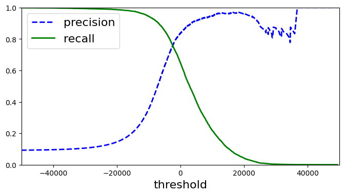
#threshold에 따른 정밀도, 재현율 plot하기 
def plot_precision_recall_vs_threshold(precisions, recalls, thresholds): 
    plt.plot(thresholds, precisions[:-1], “b–”, label=“precision”, linewidth=2) 
    plt.plot(thresholds, recalls[:-1], “g-”, label=“recall”, linewidth=2) 
    plt.xlabel(“threshold”, fontsize=16) 
    plt.legend(loc=“upper left”, fontsize=16) 
    plt.axis([-50000,50000,0,1])

plt.figure(figsize=(8, 4)) 
plot_precision_recall_vs_threshold(precisions, recalls, thresholds)
plt.show()

clf2

#재현율에 따른 정밀도 곡선 
def plot_precision_vs_recall(precisions, recalls): 
    plt.plot(recalls, precisions, “b-”, linewidth=2) 
    plt.xlabel(“recall”, fontsize=16) 
    plt.ylabel(“precision”, fontsize=16) 
    plt.axis([0, 1, 0, 1])

plt.figure(figsize=(8, 6)) 
plot_precision_vs_recall(precisions, recalls) 
plt.show() 
#재현율 80% 근처에서 정밀도 급강 - 그 전 지점 트레이드오프로 선택?

clf3

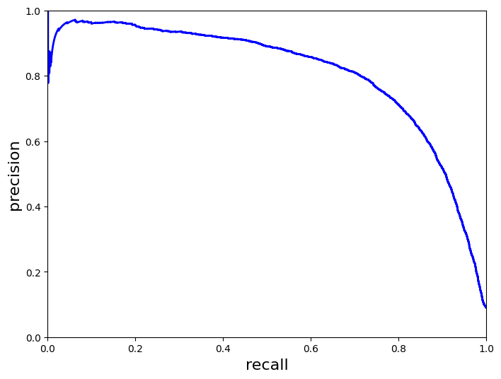
예를 들어 정밀도 90% 지점에서 트레이드오프라고 지정하면 이를 만족하는 threshold를 찾는다.

threshold_90_precision = thresholds[np.argmax(precisions >= 0.90)] 
threshold_90_precision

따라서 바로 T/F 판별대신 임의로 임계값을 설정해서 분류해 준다

y_train_pred_90 = (y_scores >= threshold_90_precision)

정밀도를 확인해 보면 90% 만족하는 것으로 나온다

precision_score(y_train_5, y_train_pred_90) 
recall_score(y_train_5, y_train_pred_90)

roc_curve

high precision, but low recall 이면 유용하지 않을것
정밀도 조정에서 재현율 - 정밀도 곡선처럼 재현율 조정을 위해 사용되는 다른 곡선
위양성비율에 대한 진양성비율(재현율) 곡선
roc_curve 함수
input = 훈련용 라벨데이터, y의 결정점수
output = 거짓양성비율, 진짜양성비율, 임계값

from sklearn.metrics import roc_curve
fpr, tpr, thresholds = roc_curve(y_train_5, y_scores)

def plot_roc_curve(fpr, tpr, label=None): 
    plt.plot(fpr, tpr, linewidth=2, label=label) 
    plt.plot([0, 1], [0, 1], ‘k–’) 
    plt.axis([0, 1, 0, 1]) 
    plt.xlabel(‘False Positive Rate’, fontsize=16) 
    plt.ylabel(‘True Positive Rate’, fontsize=16)

plt.figure(figsize=(8, 6)) 
plot_roc_curve(fpr, tpr) 
plt.show()

clf4

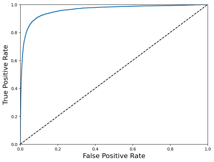
재현율이 높아질 수록 분류기의 거짓양성이 늘어난다. ROC곡선은 좋은 분류기일수록 점선에서 멀리 떨어져 있어야 한다. (점선 : 랜덤분류기의 ROC곡선)
따라서 곡선 아래 면적을 측정해서 커질수록 좋은 분류기 (완벽한 분류기 = 1, 랜덤 분류기 = 0.5)
정밀도/재현율 곡선 <-> ROC 곡선 사용하는 경우
양성클래스가 크게 적지 않은 경우 ROC곡선 -> 어느 경우든 AUC 점수가 좋으면 유용하지 않음 (반대의 경우) 거짓양성을 가려내는 것이 더 중요하면 정밀도/재현율 곡선

from sklearn.metrics import roc_auc_score
roc_auc_score(y_train_5, y_scores)

# 랜덤포레스트와 SGD 비교 - ROC 곡선 이용 
# 랜덤포레스트는 결정점수 대신 확률을 점수 대신으로 이용한다.
from sklearn.ensemble import RandomForestClassifier 
forest_clf = RandomForestClassifier(n_estimators=10, random_state=42) 
y_probas_forest = cross_val_predict(forest_clf, X_train, y_train_5, cv=3, method=“predict_proba”) 
y_scores_forest = y_probas_forest[:, 1] #양성 클래스의 확률 
fpr_forest, tpr_forest, thresholds_forest = roc_curve(y_train_5,y_scores_forest)

plt.figure(figsize=(8, 6)) 
plt.plot(fpr, tpr, “b:”, linewidth=2, label=“SGD”) 
plot_roc_curve(fpr_forest, tpr_forest, “RandomForest”) 
plt.legend(loc=“lower right”, fontsize=16)

plt.show()

clf5

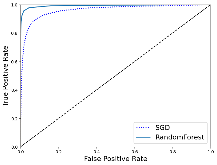
roc_auc_score(y_train_5, y_scores_forest) 
#랜덤포레스트의 분류기가 AUC값이 더 커 좋은 분류기라고 비교할 수 있다.

다중 분류

이진분류 - 5와 5아님 으로 구별한다
다중분류 - 둘 이상의 클래스 즉, 1, 2, 3 … 여러개 클래스를 구별
분류방법 : 이진분류기를 여러개 사용, 다중 클래스 분류에 이진분류 알고리즘 선택하면 사이킷런이 그에 따라 자동으로 OvR 또는 OvO를 실행한다
OvR :
OvO :

#서포트벡터머신 분류기 불러오기 
#SVC함수 fit input = X_train, y_train(label : 정수값) 
#predict 는 label의 정수값을 리턴한다.
from sklearn.svm import SVC

svm_clf = SVC(gamma=“auto”, random_state = 42) 
svm_clf.fit(X_train[:1000], y_train[:1000]) 
svm_clf.predict([some_digit])

#샘플 하나 당 10개의 결정점수 반환 - 각 클래스 분류 기준이 될 점수 
#그 중 가장 높은 점수를 가진 클래스에 할당한다. 
some_digit_scores = svm_clf.decision_function([some_digit]) 
some_digit_scores 
np.argmax(some_digit_scores) 
svm_clf.classes_ 
svm_clf.classes_[5]

#SVC에서 OvR기법 사용하는 다중 분류기를 만들고 싶을 때 
from sklearn.multiclass import OneVsRestClassifier 
ovr_clf = OneVsRestClassifier(SVC(gamma=“auto”, random_state = 42)) 
ovr_clf.fit(X_train[:1000], y_train[:1000]) 
ovr_clf.predict([some_digit])

#OvO기법 사용하도록 강제하는 경우 
from sklearn.multiclass import OneVsOneClassifier 
ovo_clf = OneVsOneClassifier(SGDClassifier(max_iter=5, random_state=42)) 
ovo_clf.fit(X_train, y_train) 
ovo_clf.predict([some_digit]) 
len(ovo_clf.estimators_)

SGD분류기는 그 자체로 다중 클래스 분류 가능하므로 그냥 실행하면 된다.
SGD에서도 decision_function()는 클래스마다 결정점수값 반환해준다.

sgd_clf.fit(X_train, y_train) 
sgd_clf.predict([some_digit]) 
sgd_clf.decision_function([some_digit])

#분류기 정확도 측정해보기 
cross_val_score(sgd_clf, X_train, y_train, cv = 3, scoring = “accuracy”)

#정확도가 더 높아질 수 있도록 X_train의 스케일 조정한다. 
#너무 오래걸려 중단… 
from sklearn.preprocessing import StandardScaler 
scaler = StandardScaler() 
X_train_scaled = scaler.fit_transform(X_train.astype(np.float64)) 
cross_val_score(sgd_clf, X_train_scaled, y_train, cv=3, scoring=“accuracy”)

위의 과정을 통해 사용하기 괜찮은 다중분류 모델을 찾았다고 가정하면 앞으로 생길 수 있는 에러의 종류들을 분석한다.

#오차행렬 측정 
#y_train_pred 에 sgd 다중분류를 실행했을 때 예측값들을 저장 
#이러한 y_train_pred의 오차행렬을 출력 (10x10 행렬) 
y_train_pred = cross_val_predict(sgd_clf, X_train_scaled, y_train, cv=3) 
conf_mx = confusion_matrix(y_train, y_train_pred) 
conf_mx

def plot_confusion_matrix(matrix): 
    ""“컬러 오차 행렬을 원할 경우”"" 
    fig = plt.figure(figsize=(8,8)) 
    ax = fig.add_subplot(111) 
    cax = ax.matshow(matrix) 
    fig.colorbar(cax)

plt.matshow(conf_mx, cmap=plt.cm.gray) 
plt.show() 
#대각선부분이 잘 분류되었다는 것을 나타내는 지표 - 밝을수록 데이터 수가 많다는 뜻 
#대각선이 어두우면 데이터의 양이 적거나 잘 분류되지 않았다는 것이라 생각할 수 있다.

clf6

각 클래스마다의 에러 비율로 비교해보자 (오차행렬 값 / 클래스당 이미지 수)
실제 클래스의 값 = row , 예측된 클래스 값 = col
8열의 색이 대체적으로 밝음 - 8 이외의 다른 이미지가 8로 잘못 분류 되었다
8행8열은 어두우므로 실제 8은 8로 분류되었다
따라서 8로 잘못 분류되는 경우를 줄이는 방향으로 조정 - 8처럼 보이는 다른 숫자 데이터로 학습시키거나 새 특성을 찾아 추가하는 방식
3, 5도 서로 잘못 분류되기도 하는 것 확인.

row_sums = conf_mx.sum(axis=1, keepdims=True) 
norm_conf_mx = conf_mx / row_sums

np.fill_diagonal(norm_conf_mx, 0) 
plt.matshow(norm_conf_mx, cmap=plt.cm.gray) 
plt.show()

clf7

#숫자그림 위한 추가 함수 
def plot_digits(instances, images_per_row=10, **options):
    size = 28 
    images_per_row = min(len(instances), images_per_row) 
    images = [instance.reshape(size,size) for instance in instances] 
    n_rows = (len(instances) - 1) // images_per_row + 1 
    row_images = [] 
    n_empty = n_rows * images_per_row - len(instances) 
    images.append(np.zeros((size, size * n_empty))) 
    for row in range(n_rows): 
        rimages = images[row * images_per_row : (row + 1) * images_per_row] 
        row_images.append(np.concatenate(rimages, axis=1)) 
    image = np.concatenate(row_images, axis=0) 
    plt.imshow(image, cmap = matplotlib.cm.binary,** options) 
    plt.axis(“off”)

clf8

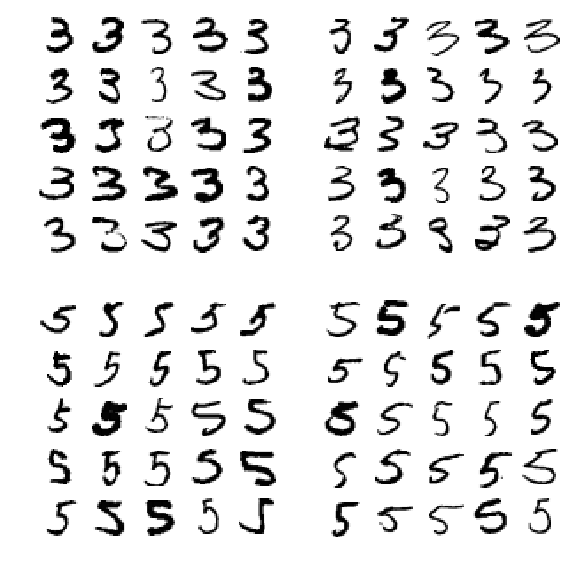
#훈련데이터중 label이 각각 3이나 5, 예측된 클래스가 3이나 5로 분류된 데이터들을 각각 경우에 따라 출력 
#label, predict 
# X_11 = (3,3) X_12 = (3,5) X_21 = (5,3) X_22 = (5,5) 
cl_a, cl_b = 3, 5 
X_aa = X_train[(y_train == cl_a) & (y_train_pred == cl_a)] 
X_ab = X_train[(y_train == cl_a) & (y_train_pred == cl_b)] 
X_ba = X_train[(y_train == cl_b) & (y_train_pred == cl_a)] 
X_bb = X_train[(y_train == cl_b) & (y_train_pred == cl_b)]
plt.figure(figsize=(8,8)) 
plt.subplot(221); plot_digits(X_aa[:25], images_per_row=5) 
plt.subplot(222); plot_digits(X_ab[:25], images_per_row=5) 
plt.subplot(223); plot_digits(X_ba[:25], images_per_row=5) 
plt.subplot(224); plot_digits(X_bb[:25], images_per_row=5) 
plt.show()

다중레이블 분류

다중레이블 분류 - 한 분류기가 샘플마다 여러개의 클래스 출력
ex) 숫자 이미지에서 1. 큰값(7,8,9)인지 출력, 2. 홀수인지 판단 - 판단은 이진분류에 해당
다중타깃 배열을 사용한다.

from sklearn.neighbors import KNeighborsClassifier 
#타깃 레이블 정하기 (T/F) 
y_train_large = (y_train >= 7) 
y_train_odd = (y_train % 2 == 1) 
y_multilabel = np.c_[y_train_large, y_train_odd]

knn_clf = KNeighborsClassifier() 
knn_clf.fit(X_train, y_multilabel)

knn_clf.predict([some_digit])

#분류기 평가하기 - 모든 레이블에서의 F1 점수 평균으로 평가
y_train_knn_pred = cross_val_predict(knn_clf, X_train, y_multilabel, cv=3, n_jobs=-1) 
f1_score(y_multilabel, y_train_knn_pred, average=“macro”)

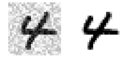
다중 출력 분류

# 다중 출력 분류 - 다중레이블 분류 + 이진분류가 아닌 다중분류 
# 이미지 픽셀 강도에 잡음 추가해주는 코드
noise = np.random.randint(0, 100, (len(X_train), 784))
X_train_mod = X_train + noise 
noise = np.random.randint(0, 100, (len(X_test), 784)) 
X_test_mod = X_test + noise 
y_train_mod = X_train 
y_test_mod = X_test

def plot_digit(data): 
    image = data.reshape(28,28) 
    plt.imsow(image, cmap = mpl.cm.binary, interpolation = “nearest”) 
    plt.axis(“off”)

some_index = 5500 
plt.subplot(121); plot_digit(X_test_mod[some_index]) 
plt.subplot(122); plot_digit(y_test_mod[some_index]) 
plt.show()

clf9

knn_clf.fit(X_train_mod, y_train_mod) 
clean_digit = knn_clf.predict([X_test_mod[some_index]])
plot_digit(clean_digit)

clf10